FastModelFree: Difference between revisions
(Added to Category) |
(LearningSorting) |
||
| Line 198: | Line 198: | ||
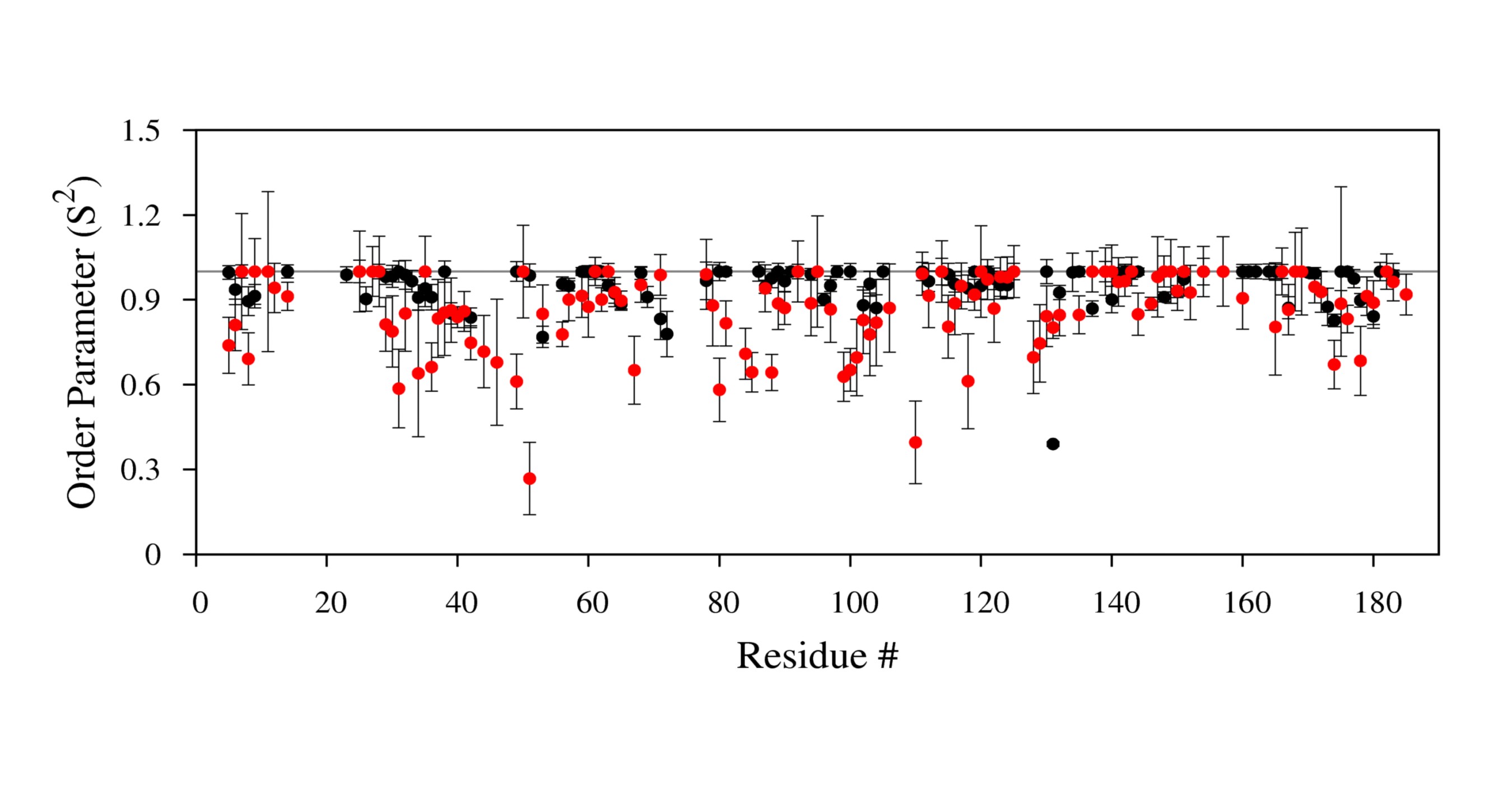
[[Image:S2plot.jpg|700px]] | [[Image:S2plot.jpg|700px]] | ||
[[category: | [[category:Protocols]] | ||
[[category:Data_Processing_and_Analysis]] | [[category:Data_Processing_and_Analysis]] | ||
Revision as of 04:50, 11 September 2021
Optimizing PDB Coordinates before using Fast Model Free
PDB Inertia
This program calculates the principal moments of inertia for the atoms in a standard pdb file.. By default the program writes the moments of inertia to standard output. Optionally, the program can output a new pdb file in which the molecule is translated so that its center of mass is located at the origin and rotated so that the moments of inertia are aligned with the Cartesian axes. At present, the program only reads lines starting with the 'ATOM' keyword and only recognizes the atoms H, C, N, O, P, S.
- Type the following command in the directory containing your pdb file
- pdbinertia -r infile.pdb outfile.pdb
- Or pdbinertia64 -r infile.pdb outfile.pdb
- This will output a translated and rotated pdb file.
R2R1 Diffusion
The program (r2r1_diffusion) uses the apprach of Tjandra, et al. [J. Am. Chem. Soc. 117:12562-12566 (1995)] to determine the diffusion tensors for spherical, and axially-symmetric motional models from experimental nitrogen-15 spin relaxation data.
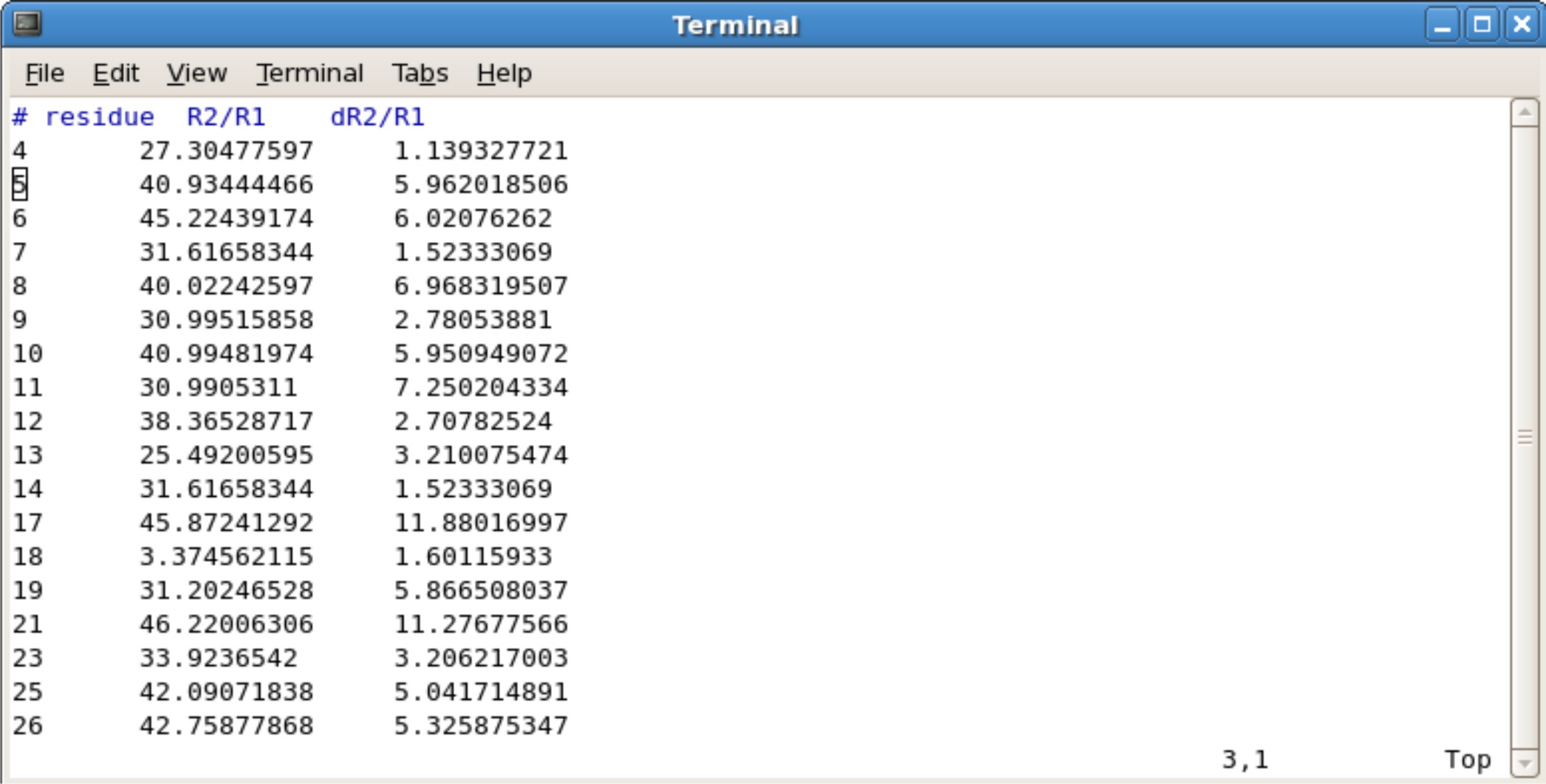
Creating R2R1 file
You will need to calculate the ratios (R2/R1) and uncertainities (dR2/R1). This can be done with any program such as excel, kaleidograph, origin, etc. The required calculations are as follows. To calculate and :
, and
The variances (squared errors) of these values are found as follows:
, and
To calculate , just divide by . To calculate the variance of that value, use:
If there is an error such as dividing by 0, remove the errors and leave blank. Save the file as a tab deliminated text file.
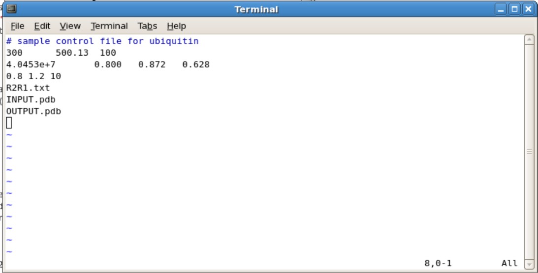
Example File
Setting up Input File
- Copy the ubq.in file into the directory containing your translated/rotated pdb file
- The ubq.in file is located in ${FMF_PATH}/r2r1_diffusion/linux
- Editing the Ubq.in
- Second Line
- The 300 represents the number of spin systems in the R2/R1 data. You will need to change this to the correct number
- The 500.13 represents the frequency of NMR you used. For example, if you use the 600 Mhz NMR, change to 600.13.
- The 100 represents the # of simulations. 100 simulations in the minimum needed.
- Third Line
- The 4.0453e+7 is your initial estimate for D-isotropic tensor. This does not need to be changed unless you have an estimate
- The 0.800 is the estimated Dpar/Dper tensor. If you do not know an estimate, set this to 1.00
- The 0.872 and 0.628 are your Theta and Phi values. If you do not know an estimate, set these values to 0.000.
- Fourth Line
- The 0.8 and 1.2 represents the predicted the High and low ratio set limits on Dpar/Dper. These values do not need to be changed.
- The 10 represents the number of steps of grid searching to be performed. This does not need to be changed. Increasing the number of steps may help accuracy, however may increase the calculation time
- Fifth Line is your R2R1.txt file
- Sixth Line is your input pdb file generated from pdbinertia
- Seventh Line is your output pdb file
- Second Line
- Running the program
- type the following command
- r2r1_diffusion ubq.in > ubq.out
- Or r2r1_diffusion64 ubq.in > ubq.out
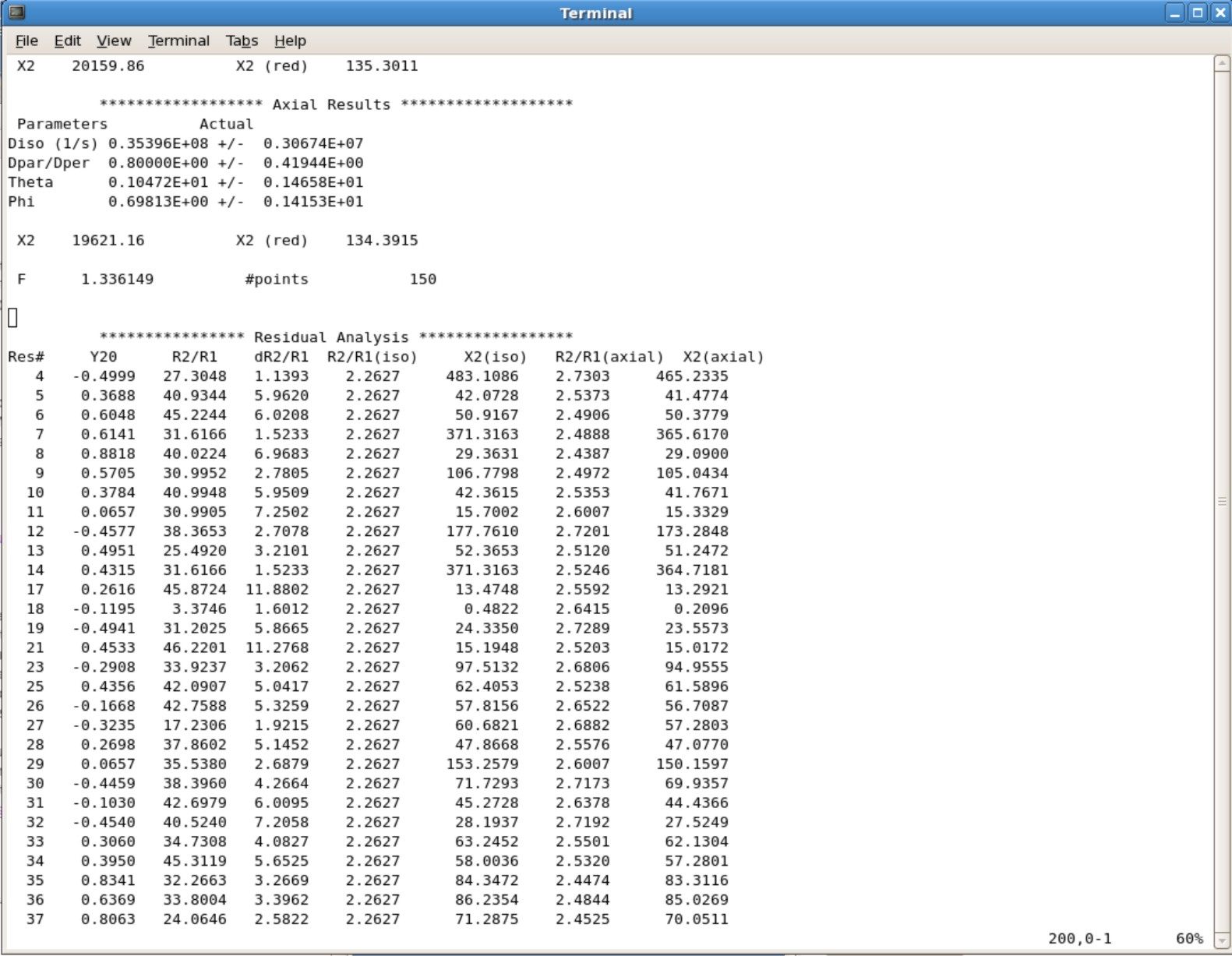
- When the program is finished, you will need to check the Dpar/Dper value
- Type vi ubq.out
- Type :$
- This will take you to the bottom of the file. Start scrolling up until you see the final parameters. Here is an example you will be seeing.
- type the following command
- If your Dpar/Dper value is the same as your minimum value or maximum value you set on the fourth line in the ubq.in file, you will need to increase the range and rerun the calculation.
- Your predicted Theta and Phi angles will be calcuated. Save those numbers to implement them into FastModelFree.
- The output pdb is what will be used for FastModelFree
Fast ModelFree
Setting up Files for FastModelFree
- You will need to copy the FMF.config into your directory containing your R2.txt, R1.txt, NOE.txt, and pdb file
- The most common problem that occurs at this point is the presence of additional white space in the input files. Make sure that additional lines after the data are deleted and additional tabs are also removed.
- FMF.config is located in ${FMF_PATH}
- You can not have more than 300 spin systems. If there is more than 300 spin systems, the program will just hang and do nothing but act like its calculating.
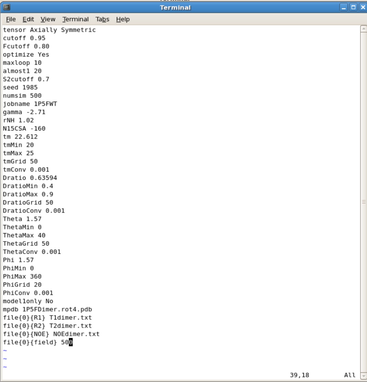
- Parameter to modify
- The manual for all the parameters are located in ${FMF_PATH}/fmfdox.pdf.
- tensor- Set as Isotropic for spherical or Axial Symmetric for non-spherical
- Make sure the A and S is capitalized for Axial Symmetric or else it will autorun as Isotropic
- You do not need a pdb file for Isotropic calculations
- cutoff set to 0.95
- Fcutoff set to 0.80
- optimize set to Yes
- maxloop set to 10. This means the program will stop after 10 iterations. If your final values have did not converge you may want to set to higher numbers such as 25 or 50 iterations.
- almost1 set to 20. You can set to higher values just like maxloop
- S2cutoff set to 0.7
- seed set to any number and change every time.
- numsim This is the number of simulation. If you want a quick and dirty estimate, you can set it to about 10 simulations. Final calculations should have a minimum of 500 simulations
- jobname set this as the name of your protein. This is the title for all your output files.
- gamma set to -2.71
- rNH set to 1.02
- N15CSA set to -160
- tm This is your predicted correlation time. If you are unsure of a correlation time, 10.0 is a good start. The farther away from the actual value the more iterations is needed and longer it takes for calculations
- You can use HyroNMR to help predict correlation time [[1]]
- tmMin Set to 0.0 if first time. You can set this min value near the actual value when you have a general idea what the tm is.
- tmMax Set to 40.0 if first time. You can set the max value near the actual value when you have a general idea what the tm is.
- tmMin and tmMax are ranges you set to believe where the actual value is.
- tmGrid set to 50. Can set to higher value for more thorough calculation
- tmConv set to 0.001 This is the convergence cutoff. You want this to be small. The accuracy decreases as you increase this value.
- Dratio This is your Dpar/Dper ratio you calculated using R2R1_diffusion calculations. You will find it in ubq.out file
- DratioMin Set the value to be smaller than your Dratio
- DratioMax Set the value to be larger than your Dratio
- DratioMin and DratioMax are your ranges you set. You want this range to be large when your first start out. After multiple attempts you can decrease the range.
- DratioConv set to 0.001
- Phi This is the Phi that you calculated using R2R1_diffusion calculations. You will find it in ubq.out file
- PhiMin set to 0
- PhiMax set to 360
- PhiGrid set to 20. Increase this value increases the thoroughness of the calculation
- PhiConv set to 0.001
- modle1only set to No
- mdpb Name of your pdb file generated from R2R1_diffusion calculations
- file{0}{R1} Name of your R1 file
- file{0}{R2} Name of your R2 file
- file{0}{NOE} Name of your NOE file
- file{0}{field} Set to 500 if using 500 MHz NMR, 600 if using 600Mhz NMR, etc.
Running FastModelFree
- To run the programs type this command
- fastMF > mf.log &
- Or fastMF64 > mf.log &
- The & symbol allows fastMF to run in the background. This process may take a minimum of 10 minutes or a few days depending how close or far away your predicted tm, Dratio, and Phi to the converged values
- You will initially see mfmodel, mfinput, mfout files, Jobname.MFDATA, Jobname.MFPAR. These files are output files generated by fastmodelfree, which are parameter sets to be used for ModelFree. The program isn't finished yet.
- You will then see your Jobname.1.pdb, Jobname.1.par. These are iterations being calculated attempting to converge all your values.
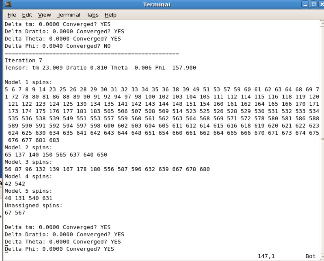
- When the calculations are finished check the Jobname.log file to see if your values converged
- The tm, Dratio, Theta, and Phi values can be found in this log file
- The Example Protein.log figure show that it took 7 iterations to for the values to converge. Protein is the protein name for the figure The correlation time, Dratio, Theta, and Phi are 23.009, 0.819, -0.006, and -157.900 respectively
- The last pdb generated is the actual pdb generated from the converged values. The name of this file would be call Protein.7.pdb, where the 7 is the 7th iteration.
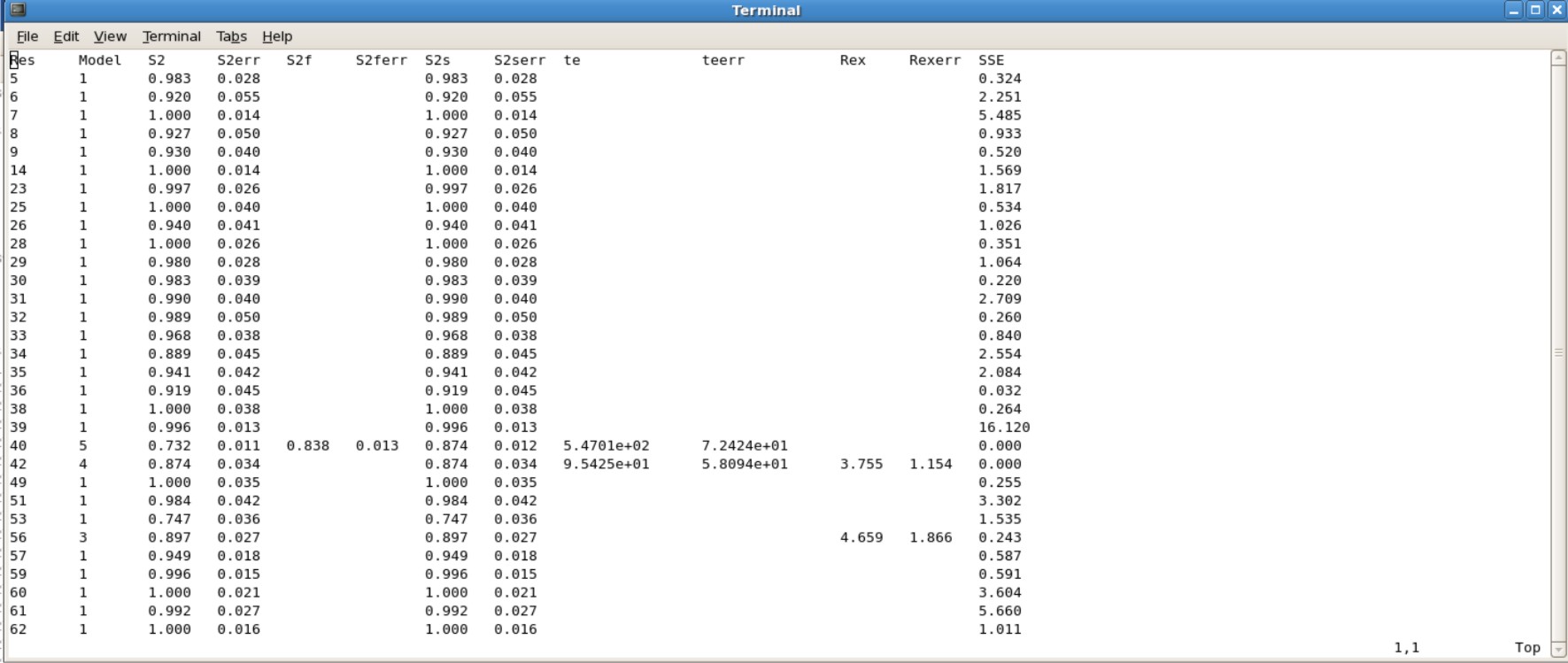
- Jobname.#.par is the results of your S2, te, Rex values. You will want to use the last .par file created. For example Protein.7.par is the actual results you want to use, in which all the value were converged.
Example Protein.7.par
Generating High Quality Graphs
Setting up Gnuplot Scripts
- Gnuplot is used to generate R1, R2, NOE, S2, Te, Rex graphs
- The files are located in ${FMF_PATH}/generate_plot
- There are 6 *.plt scripts to generate each script, and transfer them to your directory consisting of your fastmodelfree results, R1, R2, NOE data.
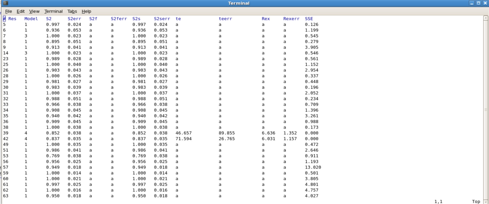
- The Jobname.#.par file consisting of your final values will need to be edited, because gnuplot does not like empty spaces in the data set. Instead you will have to insert the letter "a" in all the blank spaces. This can be done easily using excel or other programs.
- Alternatively, use the script "addA.py" to quickly insert the letter "a" into all of the blank spaces.
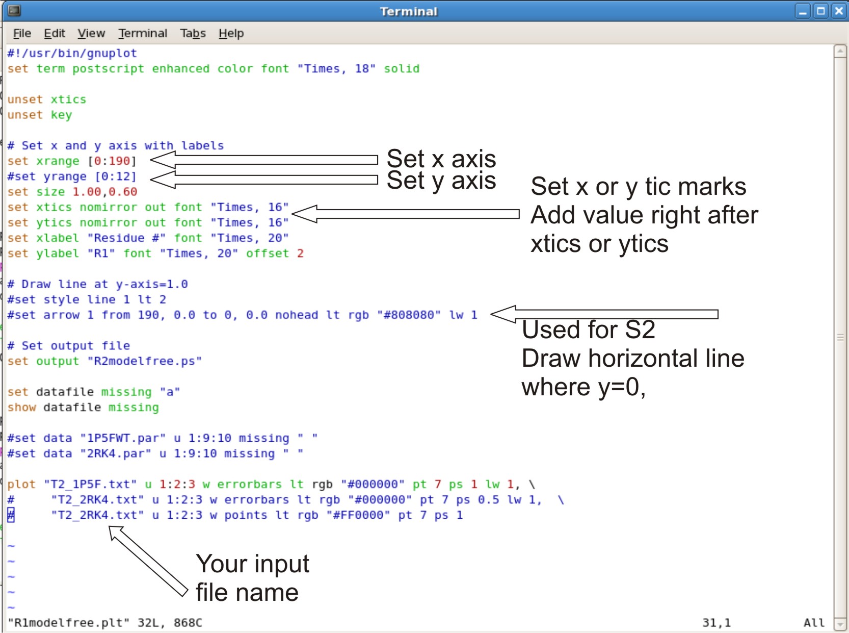
- Each .plt script will have to be edited, based on the x,y axis and input files
- Editing R2modelfree.plt, R1modelfree.plt, NOEmodelfree.plt, Temodelfree.plt, Rexmodelfree.plt, s2modelfree.plt
- set your xrange as [0: #ofresidue + 2] Adding +2 to x range will allow the last point to be in the graph instead at the edge
- setting yrange. This is normally commented out (ex.adding # at beginning of line). This allows the y range to be to be set up automatically.
- If the graph looks bad at y range, Take out the # sign. Change the numbers in the bracket to the range you want. example [0:12]
- setting xtic or ytics. The tics are normally setup automatically.
- If you do not like the range of tic set up. You can set your own tic range
- example: xtics 3.0 nomirror out font "Times, 16". The 3.0 set the tic range at 3.0 values apart, therefor you will see a tic at 3.0, 6.0, 9.0.
- If you do not like the range of tic set up. You can set your own tic range
- Setting up horizontal line where y=0. This is for s2modelfree.plt only
- Where is says set arrow 1 from 190. Change the 190 to the max range you set for your x axis.
- Setting up your input file
- At the bottom of the script where it says plot
- The script is designed to compare two different plots, where there is 3 lines involved.
- The first line is the data for your first protein. The second and third line is the data for your second protein. If you only have on protein data set, you can comment out the second and third line with a # sign at the beginning of the line.
- For R2modelfree.plt use R2.txt data
- For R1modelfree.plt use R1.txt data
- For NOEmodelfree.plt use NOE.txt data
- for Temodelfee.plt, rexmodelfree.plt, and S2modelfree.plt use edited Jobname.par generated by modelfree
- At the bottom of the script where it says plot
Running Gnuplot Scripts
- To run the program, type the name of .plt file to run it.
- example: Type R2modelfree.plt to create R2 graph.
- a .ps file will be generated which contains your graph.
- to generate a pdf. Type pstopdf filename of graph


